
. Introduction
Deformation analysis aims at inferring on geometrical changes of objects under study. The object, in fact, may be of material character, for example, deformation of the Earth’s crust, and also may have an abstract character, for example, deformation of the gravity field (Dermanis and Livieratos, 1983). Both cases are treated by the same tools originating from, for example, differential geometry, theory of elasticity (also continuum mechanics), estimation theory, and tensor calculus. The geometrical changes are understood as rigid motions and distortions of the object’s shape. Deformation analysis has a very broad spectrum of applications in seemingly not related fields but aiming at as accurate as possible description of object’s behavior in different time instances (epochs). It is used, amongst others, in biomechanics and medicine-related applications (Tanaka et al., 2012; Bayly et al., 2005), in surveying engineering (Caspary et al., 1990), in Earth’s crust movement monitoring (Altiner, 2013; Dermanis and Kotsakis, 2006), and in landslides monitoring (Szafarczyk and Gawalkiewicz, 2016) to mention only a few.
The search for simple and universal methods (and also software development) for the determination of a deformation field is still an up-to-date research topic Goudarzi et al. (2015). In this article, we present a simple method to approximate a deformation field based on the tools that surveyors and geodesists are familiar with. It uses a distance-weighted affine transformation model performed in a local manner and calibrated in a cross-validation (CV) procedure. The method uses a rigorous approach to recover a rotation and a stretch tensor from a deformation gradient. This approach relies on the use of polar decomposition of a deformation gradient rather than the use of simplified decomposition into symmetric and skew-symmetric parts. However, the two are discussed. The use of the latter mentioned decomposition was justified when the computer processing power was limited or it may be accepted when a priori knowledge of small rotation angles is present. The method provides all estimated quantities (strains and rotation) with their standard errors obtained via variance–covariance propagation law.
The article is organized as follows. The first introductory section defines quantities that are used throughout the article, that is, a deformation gradient (or displacement gradient), the polar decomposition of a matrix (used to separate rigid rotations from deformations), and two strain tensors. The second section shows the mechanics of the method. It presents the affine transformation model in its explicit (geometric parameters equal to rotation and strain tensor entries) and implicit (transformation parameters) forms. It also demonstrates the use of polar decomposition to recover geometric parameters from transformation parameters. In addition, a formula based on the variance–covariance propagation law for error analysis of the geometric parameters of the transformation and a CV technique to calibrate the local affine transformations are presented. The next section is a part of numerical example. Data are simulated to have the full control over the method. The data generation process is explained, and necessary formulas are provided. The subsequent section shows the results of the method and its reliability in comparison to theoretical values of generated deformations. Finally, conclusions are drawn.
. Deformation Gradient, Polar decomposition, and Strain tensors
Deformation gradient (F) or/and displacement gradient (G) are basic tools while analyzing deformations (in theory of elasticity and continuum mechanics). If we introduce two configurations of points (homological) representing any object and we denote a vector of coordinates of any point in the first one as x = [x y]T (initial or reference) and in the second one as X = [X Y]T (current or deformed), then we may try to define a relation between x and X of the form X = f(x). The deformation gradient is defined as the derivative of each component of the deformed X vector with respect to each component of the reference x vector. Hence, the deformation gradient (here in 2D) reads as follows:
On the other hand, if we introduce a displacement vector u = X – x, then the deformation gradient may be expressed as
where
To recover deformations and rotations from the deformation gradient, a polar decomposition is used. The polar decomposition of a matrix factorizes the matrix into a product of an orthogonal matrix R and a symmetric positive (semi) definite matrix U (a stretch tensor), that is,
where R must obey det(R) = 1 to be a rotation matrix. The polar decomposition may be obtained, for example, by means of singular value decomposition (SVD) or spectral decomposition. Generally, in order to transform a stretch tensor U (factor of the polar decomposition) into a strain tensor, one subtracts the identity matrix from it (or takes its logarithm, i.e., logU, but this strain measure will not be used in this work) for the review of these mentioned and other strain measures, for example, see Chaves (2013). In this work, we use only two strain measures (tensors):
i. Biot’s strain tensor (a straightforward measure of strain but not commonly used):
ii. Small (engineering/infinitesimal) strain tensor (common but limited to small rotations):
Using polar decomposition with R = I (no rotation case), that is, F = RU = U, it is easy to show that the small strain tensor is identical to Biot’s tensor:
For negligible rotations, not the strains themselves, instead of the polar decomposition, one may use a simple decomposition of a displacement gradient into a symmetric matrix (eq. (5)) and a skew-symmetric one, that is,
where Gs (a symmetric matrix) stores information on expansion, contraction, and shearing deformations at a given point and Ga (a skew-symmetric matrix) carrying information on rotations (infinitesimal ones) (Berber et al., 2012).
. Mechanics of the method
. Affine transformation
To locally relate coordinates of an undeformed (reference, initial) configuration (or configuration obtained from any previous measurement), denoted in lowercase, with the coordinates of deformed configuration (current or final), denoted in uppercase, we use affine transformation model, known also as 6-parameter transformation. The affine transformation is a simple and flexible model (deforms shapes but parallel lines are preserved) often used in surveying and mapping practice. For a single point, we construct two equations of the following form (e.g., Osada and Sergieieva (2010)):
or in a matrix-vector form:
where tX, tY , sx, and sy are translations and scale factors (stretches) along the x- and y- axes, respectively; sxy is the shear; and ’ is the rotation angle while transformation parameters a, b, c, and d are functions of previously introduced geometric parameters. To solve for unknown parameters, we need at least three homological points in no adjustment case or more to adjust the results and obtain some accuracy measures. Equations (8a), (8b) or (9) reveal the relation among transformation parameters a, b, c, and d and geometric parameters sx, sy sxy, and φ. The considered model is nonlinear with respect to geometric parameters (scale factors, shear, and rotation), and it can be solved through linearization and iteration to explicitly obtain geometric parameters (rather uncomfortable solution). On the other hand, this model is linear with respect to transformation parameters and may easily be solved in the linear least squares framework (this option was chosen in this work), but this will require a variance–covariance propagation from transformation parameters to geometric parameters (shown hereafter). The local affine transformations are weighted, in this work, by means of inverse distance squared between each grid point (new point) and observed points (nearest neighbors). It is easy to notice that the deformation gradient and its polar decomposition in the affine transformation case read (compare to the right hand side of eq. (9)):
. Polar decomposition (once more)
Polar decomposition of a matrix is very often presented and computed via abovementioned SVD. Using SVD to extract a rotation matrix and a stretch matrix (stretch tensor) from the
deformation gradient, we have the following relation:
where W and V are orthogonal matrices and Σ is a diagonal matrix with non-negative values on the main diagonal. By introducing the product VTV before Σ in (11), one obtains
Hence, the factors of the read as
A firm review of polar decomposition algorithms (iterative and exact) and its properties may be found in, for example, Gander (1990), Markley and Mortari (1999), Higham (1986), Shoemake and Duff (1992).
. Variance and covariance propagation among transformation parameters and geometric parameters
To equip the geometric parameters (obtained with the use of polar decomposition) with standard errors, the variance–covariance propagation law was used. According to equation (8a), (8b) or (9), transformation parameters may explicitly be expressed as functions of geometric parameters, that is,
Jacobi matrix reads as (the order of differentiation is tX, tY , sx, sy, sxy, φ)
(15)
If we denote a vector of transformation parameters as
and a vector of geometric parameters as
then the variance–covariance propagation law gives
and standard errors are the square roots of entries on the main diagonal of the matrix (18).
. Calibration of the model
Calibration of the model means here selection of optimal number of nearest neighbors (or possibly other factors influencing the model) for local affine transformations. The model is calibrated on known points (observations) with an assumption that the results of calibration should be valid for all points within a study area. As a criterion we use, a CV score that is equal to
where
N denotes the number of known points. The lowest value of CV score indicates possibly the best model among the tested (optimal in CV-sense number of nearest neighbors or other parameters defining the model).
. Data
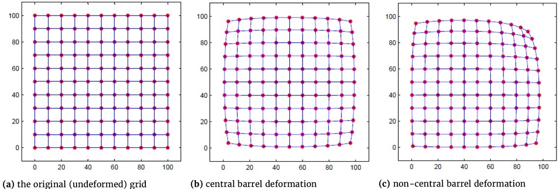
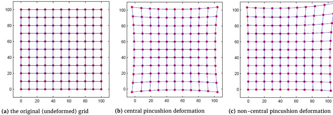
In order to have full control over the operation of the method, the deformed grids (a current configuration) on the basis of undeformed ones (a reference configuration) have been simulated in a functional manner. They were generated according to the swirl-like (Fig. 1), barrel (Fig. 2), and pincushion (Fig. 3) deformation models. Thus generated grids acted as observed points (with known coordinates in current and reference configurations). The grids were generated in a regular (equally spaced points) and irregular (percentage of randomly deleted points from the regular grid) manner (irregular ones are not presented in the figures). Only the kinds (shape) of deformation used in this study are demonstrated in the included figures.
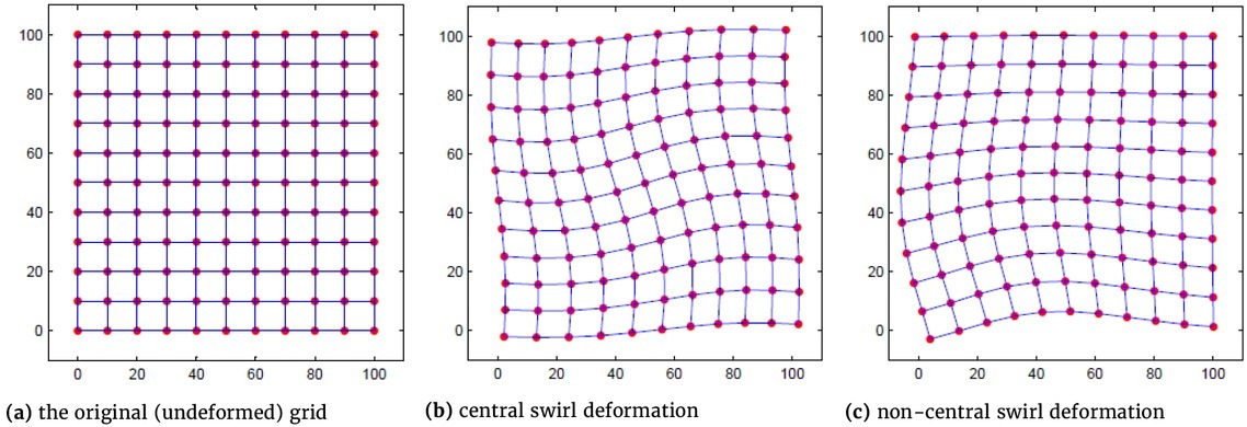
. Swirl-like deformation
Swirl-like deformation is introduced by the following formulas:
where
Components of the deformation gradient, given in (1), in this case read as
. Barrel and Pincushion deformations (distortion)
where
. Results
In this section, some exemplary results from simulation study of the method are presented. Tables 1–3 present selected results for above-described deformation models. As measures of deformation structure recovery, we used minimum value, 1st quartile, median, 3rd quartile and maximum value, mean error (ME as a measure of over- or underestimation), mean absolute error (MAE), and a correlation coefficient between true and estimated strain components. ME and MAE are based on differences between corresponding true and estimated values of strain tensor components. In all presented cases, strain components were determined at points being incenters of Delone triangles covering the simulated study areas. Five nearest neighbors were used to generate locally weighted affine transformation models giving the opportunity of providing the results with error analysis. A spatial domain of 500 m × 500 m was covered by regular and irregular grids of points. The regular grids consisted of 10 points in each row and in each column (100 points). In order to keep the same number of points for irregular grids, a densified set of points (20 in each row and column) was generated and then 75% of points were randomly removed. Simulated deformations resulted in various (from low to high) magnitudes of displacements of grid points.
Table 1
Comparison of statistical measures for true and estimated strain components for regular grid (first rows) and irregular grid (second rows) in a central swirl-like deformation model
As first, the results from a swirl-like deformation with significantly varying displacements will be presented (extreme case). The results from both regular and irregular grids will be presented in a single table; in every cell, the first row refers to the regular case and the second row refers to the irregular case (this also concerns remaining deformation models).
The results contained in Table 1 concern data generated according to a central swirl-like deformation with parameters: x0 = mean(x), y0 = mean(y), α = π/50, and b = 100. These parameters resulted in displacement of points varying from - 2.4318 to 2.4318 m (with arbitrary intermediate values) with respect to the reference (undeformed) configuration. Comparison of statistical structure of true and estimated strain components (for both grids) measured by minimum value, maximum value, and quartiles reveal moderate but still very informative correspondence between the two. Values of MEs, on the other hand, reveal negligible overestimation (underestimation) in this case. Correlation coefficient for the regular grid close to unity confirms a linear relationship (correspondence) of true and estimated strain tensor components. Also MAEs prove satisfactory accuracy obtained from the method in this case. It is worth mentioning that absolute differences between true and estimated strain components do not exceed (in majority of points – 90%) values of corresponding standard errors offered by the method (eq. 18). For irregular case, a decrease in structure recovery is visible. MEs reveal stronger underestimation (overestimation) of strain tensor components; MAEs are roughly 2.5 times larger than those in the previous case. Correlation coefficient, although visibly lower, is still close to unity and confirms a linear relationship (correspondence) of true and estimated strain tensor components. This accuracy degradation is justified by large deformations (generated on purpose) manifesting themselves by points’ displacements and irregularity of sampling.
Table 2 contains the results for a non-central barrel deformation with parameters x0 = 0.45•mean(x), y0 = 0.45•mean(y), c1 = –5 • 10–15, c2 = –5 • 10–15. These parameters resulted in displacement of points varying from -0.1747 to 0.0149 m (balanced in comparison to the previous deformation model) with respect to the reference (undeformed) configuration.
Table 2
Comparison of statistical measures for true and estimated strain components for regular grid (first rows) and irregular grid (second rows) in a non-central barrel deformation model
Table 3
Comparison of statistical measures for true and estimated strain components for regular grid (first rows) and irregular grid (second rows) in a non-central pincushion deformation model
The estimated quantities match theoretical ones accurately. Values of MEs reveal insignificant overestimation in this case. Correlation coefficients close to unity confirm a linear correspondence of true and estimated strain tensor components. MAEs prove more than satisfactory accuracy obtained from the method used in this case. The results listed in Table 3 concern data generated according to a non-central pincushion deformation with parameters x0 = 0.75 • mean(x), y0 = 0.75 • mean(y), c1 = 5 • 10–15, c2 = 5 • 10–15. These parameters resulted in displacement of points varying from -0.0165 to 0.0596 (mild) with respect to the reference (undeformed) configuration.
Also in this mild-deformation case, one observes very good strain tensor structure recovery with regard to its theoretical counterparts. The results are so satisfactory that they do not require further comment.
As mentioned in the introductory section, the use of small strain tensor (eqs. (5) and (7)) in deformation analysis is justifiable when there is no rotation or it is negligible. The last two simulations are very good examples in this respect because these deformation models do not contain the rotation component at all. Hence, in these cases, there is no difference between strain tensor components obtained by means of eqs. (4) and (5). On the other hand, for a swirl deformation model that consists of variable rotations, the difference between the two strain tensors becomes visible, although the presented example uses rather small values of rotation angles. Maximum difference between the small strain tensor and Biot’s strain tensor reaches the value of 1.8 mm/m (for 3.4° rotation angle), and also significant differences are observed for angles down to approximately 1.5•. Comparing the maximum difference between the two tensors with the overall accuracy of the method measured by MAE, one notices that the magnitude of this difference exceeds the MAE for the regular grid and makes approximately 65% of MAE for irregular grid (for particular values, see Table 1). Hence, when a rotation component is not negligible, the use of small strain tensor is a misuse and may lead to unreliable results. Generally, with readily available modern computer power at hand, there is no need to use simplified solutions; hence, the use of polar decomposition is recommended. The use of this decomposition is not computer intensive because we use only 2nd-rank tensors represented by matrices (2×2 for 2D and 3×3 for 3D).
. Conclusions
In the article, we have presented a simple method that approximates a planar deformation field, that is, strain tensor and rotation components. The method is based on a distance-weighted affine transformation model performed for each generated grid point based on the nearest observations covering the study area. In order to recover a stretch (and later a strain) tensor and a rotation from local affine transformation parameters, we used a standard tool used in continuum mechanics, that is, the polar decomposition performed with the use of another matrix decomposition, that is, singular value decomposition. The latter decomposition is easily accessible in many software packages, for example, MATLAB, Mathematica, Mathcad, R, and others. For comparison purposes, we also used a simplified decomposition, that is, decomposition into symmetric (strain) and antisymmetric (infinitesimal rotation) parts. The comparison demonstrates that when a rotation component is not negligible, the use of small strain tensor may lead to unreliable results. To perform accuracy analysis, we also derived a formula for a covariance matrix for stretch (also strain) and rotation tensors components. The derived formula is based on a variance–covariance propagation law between affine transformation coefficients and geometric parameters. Many numerical (simulation) tests (among them, those presented in the content of the article) proved the potential and usability of this simple method in deformation-analysis-related problems. The method may be extended to a 3-dimensional case what is in fact in progress. In the simulation study, we omitted all issues concerned with eigen (spectral) analysis of strain tensors because it would not bring any additional information to the presented method in the context of this article.