. Introduction
At present, the methods of using UAV are being intensively developed. These technologies have a number of advantages: they don’t require specially prepared platforms and launcher, they are relatively inexpensive unlike large aircrafts, they are safe. UAVs of winged or plane type gained the greatest development and distribution in the world. Modern UAVs have a wide range of capabilities, beginning from surveying in the visible spectrum, finishing with thermal and lidar surveying. If you consider the possibility of using the UAV for monitoring, then there are fairly large prospects for the development of these technologies.
The application of the UAV has many advantages: profitability, the possibility of surveying from low altitudes near objects and obtaining high-resolution images, speed in taking pictures, possibility of using in emergency zones without risking life and health of pilots. The UAV must have a full autopilot on the board capable to control surveying parameters (route, inclination angles of the digital camera, the corresponding percentage of longitudinal and cross overlapping, height), even with a small mass of the device in the wide range of meteoconditions.
UAVs are divided by the type of control on manual (from the remote control panel within optical observation), automatic (with the use of onboard software devices on the given trajectory, on the assigned altitude, with the assigned speed and with stabilization of orientation angles) and semi-automatic (autonomous flight with the operator’s ability to make changes into the route). The last two ways are the most demanded today by the users of unmanned systems, as they have the few requirements to personnel training and provide safe and effective operation of unmanned aerial vehicles.
Completely automatic control helps to facilitate the solution of the problem of aerial photography of a given area when it is necessary to research at a great distance from the place of basing out of contact with the ground station. For the realization of digital aerial photography, the UAV should be considered in conjunction with its equipment and payload, for what the term unmanned aerial system (UAS) is introduced, which except the UAV, consists of an on-board control system, payload and a ground control station.
While designing a UAV, various approaches are proposed to reduce the inclination angles by stabilizing UAVs. In particular, using linear quadratic regulators successfully solve this problem by hanging, but don’t work with significant non-linear and cross links (Santos et al., 2013). You can use a replaceable control mode, which is simple and reliable, but it requires adaptation of switching logic to flight modes (Li et al., 2013).
The publication Gong et al. (2012) developed an algorithm for tracking the UAV trajectory based on the PD controller and the ‘backstepping’ method with a corrective filter. The works Dierks and Jagannathan (2010); Xian et al. (2015) propose a nonlinear controller based on a neural network, and in Yi et al. (2014) – a real-time algorithm for trajectory planning and collision avoidance. Roberts and Tayebi (2011) considers an adaptive position tracking algorithm for vertical take-off and landing with limited external disturbances.
In the article Melnikov et al. (2012), a study was conducted using a MEMS accelerometer and a low-price gyroscope to determine the angular position of the UAV (angles of roll and pitch). The task was carried out with the help of the micro-controller AVR A Tmega 16 with the algorithm of the optimal Kalman recursive filter incorporated in it. The device proposed by the authors determines the angles of roll and pitch with errors ±1°–3° in the steady state, and ±3°–10° in the dynamic mode. The range of measuring the roll angles is ±175° and the pitch angles is ±90°. It should be noted that about 60% of the flights of a small aircraft are carried out according to the rules of visual flights. Therefore, taking into account the low price (~100 $), the use of the device proposed in the work is very promising in terms of improving the flight’s safety. The device in combination with a PID controller can be used to stabilize the angular position of objects.
In Andropov et al. (2016), the problem of stabilization of a multi-rotor UAV under the conditions of unaccounted perturbations is investigated. The classical PID controller is considered. Method for adjusting the coefficients of an adaptive PID controller based on neural networks is proposed. The structure of the neural network, its input and output data are investigated. To create an adaptive stabilization system for multi-rotor UAV, neural networks with three layers of trainees using the back propagation error method were used. As a result of the operation of neural networks, the coefficients for the regulator are determined for any case of stabilization. The above method of adjusting the coefficients can be used in the management of unmanned aerial vehicles operating under conditions of the changing external environment.
The publication Gen and Chulin (2015) proposes an algorithm for stabilizing the UAV flight and explores the possibility of applying this algorithm to trajectory control. Quadrocopter mathematical model is constructed, the model is verified with comparative modelling in Matlab Simulink and Universal Mechanism software systems. The development of the controller, which allows to stabilize the altitude, angular position and control the trajectory of the flight of a quadrocopter is presented. The simulation results show satisfactory stability of the quadrocopter flight and tracing of the specified trajectories, confirms the correctness and validity of the control algorithm.
In the paper Varzanosov and Solodkiy (2016), the stabilization one-coordinate platform system based on a stepper motor is considered. Components that meet the requirements of stabilization were studied and selected. MEMS sensors were used to reduce the weight of the system and thereby increase the battery life.
Presented literary sources about the stabilization of all types of UAVs are only a small part of the publications devoted to highlighted topics. Therefore, the problem is really relevant and it is important to investigate all possible factors affecting the stability of a UAV flight. However, for ultralight UAVs, there are still many unsolved problems, especially when performing aerial photography. The aerial photography requirements are fairly rigid; first of all, the inclination angles should not exceed 3–5 degrees, since this will affect the accuracy of determining the coordinates of the points of objects. Therefore, this publication presents the results of the study of correlation between angular elements of exterior orientation with each other, in order to take into account this fact for the processing of aerial photographs.
. Purpose and method of development
The purpose of the study is to determine the correlation between the angular elements of exterior orientation.
Between the functional dependence and the complete independence of the variables, there is a range of association that are called correlation. In contrast to the functional dependence, the correlation reflects the relative connection. The correlation relation can be conditionally described by the equation:
where f(x) – part of the resultant characteristic, which was formed under the influence of the accounted, known factors, which are in correlation with y; " – part of the resultant characteristic, which arises as a result of the action of unaccounted factors.
The general method testing the hypothesis about correlation existence between the variables involves three stages: the definition of the type of data, the verification of the hypothesis about the absence of relationships, the assessment of the strength of the correlation. The type of output data significantly influences the choice of methods and criteria that can be applied in the next stages of the analysis.
For the preliminary assumption about the presence and type of connection between certain variables, it is expedient to bring the data into correlation tables and construct a correlation diagram.
Pearson correlation coefficient is calculated to determine the strength of linear association
where x̄, Ȳ – mean values of variable x and y, respectively.
Value ryx close to -1 or +1 indicates the presence of a linear relationship between the variables. The approximation of its value to 0 indicates the absence of a linear association, but is not a proof of the absence statistical connection. For data sample n > 50, the significance of the linear connection is checked by the Romanovsky criterion: if
If there is a non-linear relationship between the sets of data, then the correlation ratio (square root of the ratio of the factor variation of the quantity to its general variation) is often used to estimate the degree of association strength [Bakhrushyn, 2011]:
where n – number of observation, m– number of groups, νj – number of data, which were caught in the j-th interval of the grouping, yji – value of the i-th observation of the investigated characteristic, which were caught in the j-th interval.
The zero value of the correlation ratio corresponds to the absence of any connection. Values ηyx close to 1 indicate the presence of a nonlinear dependence. It should be noted that the grouping of data can be carried out in various ways, so there is a certain underdetermination of the correlation ratio. However, this is an empirical indicator of the association strength, which differs from the linear one. If ηyx = |ryx|, then there is linear correlation between y and x, or it does not exist at all. If ηyx > |ryx|, then this can be a proof of a nonlinear connection presence. This fact makes it possible to use the difference ηyx and ryx as a characteristic of the deviation of the correlation from the linear one. For this purpose, the value ν2 is calculated:
where n– number of the empirical points, k – number of the groups. This quantity obeys an F-distribution with parameters k–2 and n–k. If the value calculated by the formula (6) exceeds the point
In addition, based on the grouped data, it is possible to construct empirical regression lines that show how the characteristic y changes with increasing x and helps to define a form of the relationship between the quantities. The form of the correlation between random variables and the resulting value is called the regression equation. There are pair and multiple regressions of linear and nonlinear types. The form and parameters of the regression equation are found using the method of least squares. The quality of the regression model is assessed using the F-test (Fisher-Snedecor criterion).
. Results
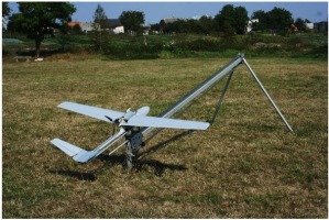
To investigate the association between the angles of pitch α, roll ω and yaw ĸ a sample of 100 units was used. This data was obtained from the file of recordings of the UAV ‘Arrow’ aircraft type, developed and created by specialists of National
University Lviv Polytechnic and the company ‘Abris’ (Fig. 1). Specifications are presented in Table 1.
Table 1
The technical characteristics of the UAV ‘Arrow’
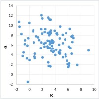
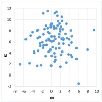
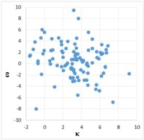
Based on these data, correlation tables and correlation diagrams were constructed (Fig. 2– 4).
As we can see, the experimental data are quite scattered, but some of the points are located close to each other and form the core. There is a tendency of decreasing of the variable with the growth of the attribute (Fig. 2).
The values of the Pearson correlation coefficient, calculated according to formula (1) for each pair of values are as follows: rĸα = –0.364, rαω = 0.051, rĸω = –0.138. Since the correlation coefficient for the quantities α and ω is very close to zero, we can therefore assert that there is no linear relationship between the quantities. Value rĸω indicates a weak inverse linear relationship and rĸα indicates a moderate connection. The verification of the significance of the linear association for these coefficients according to the Romanovsky criterion led us to the conclusion that there is no pairwise linear relationship between the values α andω, ĸ andω, and there exists a moderate connection between ĸ and α.
Subsequently, the initial data were grouped into 8 groups for each pair and the mutually-conjugate empirical correlation ratios for each pair of characteristics were calculated using formulas (3)–(5): ηĸα = 0.33 and ηαĸ = 0.35; ηαω = 0.3 and ηωα = 0.22; ηωĸ = 0.26 and ηĸω = 0.37.
For values ĸ and α, rĸα ≈ ηĸα that can be a proof of linear relationship between them. Since rest of the correlation relations exceed the corresponding linear correlation coefficients, this may indicate a nonlinear relationship between the angles of pitch, roll, and yaw. Let’s check the hypothesis about the linearity of this connection by the F-distribution. Consequently, k – 2 = 8 – 2 = 6 and n – k = 92 , the critical point of the
F-distribution (6; 92)
According to the grouped data, using the group mean, we constructed the so-called empirical regression lines (Fig. 5), which shows how the dependent variable changes with increase in the factor quantity. We see, however, that there is no relationship between ω and α, and for the rest of the pairs of quantities, there is already some inverse dependence.
Obtained results lead to the thought about very weak correlation between the angles of pitch, roll and yaw. However, the correlation coefficients that we have calculated don’t take into account the indirect or joint effect of the remaining values, then the assumption about connection existence between the pitch, roll and yaw are not completely rejected. We continue research using multiple correlation-regression analysis. The resulting paired correlation coefficients rĸα = –0.364, rĸω = –0.138 and the corresponding empirical regression lines led us to the idea of investigating the combined influence of factors α and ω on the yaw angle ĸ. To do this, we calculated the coefficient of multiple correlation R and the parameters of the linear regression equation ĸ = a0 + a1α+ a2ω following using the least squares method in the Excel spreadsheet that uses a statistical data analysis package. The results are presented in Tables 2–4.
Table 3
Parameters of the regression model
Table 4
Dispersion analysis
| df | SS | MS | F-value | Significance level F | |
|---|---|---|---|---|---|
| Factors (m) | 2 | 1046.16831 | 523.0841551 | 7.937286751 | 0.000649162 |
| Residue | 95 | 6260.70297 | 65.90213653 | ||
| n – m – 1 | 97 | 7306.871281 |
Here, t-statistic – ratio of Coefficients and Standard Error, P-value – significance for t-statistic, Lower 95%; Upper 95% – confidence interval for coefficients of regression model, df – the number of degrees of freedom, SS – dispersion (factor, residual, general), MS – ratio of dispersion and number of degrees of freedom, F-value – assessment of the relationship between independent factors and the dependent variable, Significance level F– lower level shows better connection.
So, according to Tab. 2, the multiple correlation coefficient R = 0.378, which indicates a moderate relationship between the score ĸ and factors α andω, and also the presence of additional unaccounted factors of influence.
The equation of dependence (regression model), in accordance with Table 3, has the form ĸ = 4.482 – 1.233α – 0.248!. As we can see, roll angle ω and pitch α have an inverse relationship with the yaw ĸ, since the coefficients of the equation are negative. The most significant factor is the quantity α (the value of the t-statistics is above the critical value tk = 3.3 for k = 100–2 and the significance level of 0.001). Sufficiently large value of the free term a0 = 4.482 in the regression equation indicates a significant influence of other unaccounted factors on the magnitude of the yaw angle. The last two columns of the Table 3 provide limits of confidence intervals for the coefficients of the regression equation with a significance level of 0.05.
To evaluate the quality of our regression model, we use the Fisher criterion. The value F = 7.937 is from the Table 4 with a significance level of 0.001. Critical value of the F-test is Ft(0.001; 2; 97) = 4.9. So, since F > Ft, our regression model is statistically reliable with a significance level of 0.001.
The resulting regression model allows to assert that angular
elements of exterior orientation are correlated with each other. Therefore, in further image processing, it becomes possible to make compensation of this fact and to improve the calculation accuracy of the points’ spatial coordinates on the images.
. Conclusions
As a result of our research, we have made the following conclusions:
The dependence between the pitch α, roll ω and yaw ĸ angles is investigated with the purpose of further reducing the influence of the inclination angles on the resulting images. This fact, in turn, will increase the accuracy of creating large-scale plans and orthophotomaps and will make it possible to create topographic plans of even larger scales (1:200–1:100) using UAV as a promising topographic tool.
Based on the data obtained from the UAV autopilot record file, correlation diagrams for the pitch α, roll ω and yaw ĸ angles were constructed.
Correlation coefficients and empirical correlation ratios between the angular elements of exterior orientation were calculated. According to grouped data, we constructed empirical regression lines. The obtained results indicated a moderate relationship between the investigated values.
The calculated value of the multiple correlation coefficient indicated moderate joint effect values of ω and α on the value of the yaw angle ĸ. Founded parameters of the linear regression equation testified about the inverse relation between the quantities and indicated that a more significant factor of influence on the value of ĸ is the change in pitch angle α. In addition, the value of the free term in the regression equation indicated a large influence of unaccounted factors on the value of the yaw angle ĸ.
The resulting regression model allows to assert that angular elements of exterior orientation are correlated with each other. Therefore, in further image processing, it becomes possible to make compensation of this fact and to improve the calculation accuracy of the points’ spatial coordinates on aerial photography images


