
. Introduction
Today, area data is a basic parameter derived from analyses required for a large number of decision-making processes. The area needs to be calculated correctly because the values obtained as a result of calculations have an effect on cost. The values obtained as a result of area calculation are used in many fields such as engineering applications, geodetic studies, cadastral studies, zoning and expropriation applications, land valuation activities, forestry, agriculture and taxation. In such activities, Geographic Information Systems (GIS) are frequently used to obtain information such as cost–benefit analysis. Users obtain the area data of a parcel from the land register, land measurements or by digitisation from a scaled map. In any case, the area value is calculated from two-dimensional maps, in other words, the plane geometry. Maps are produced based on reference surfaces such as three-dimensional ellipsoid or sphere closest to the geoid using projection or map methods. In order to calculate the exact area value of a parcel on the map, area corrections must be added to the area value calculated on the map (Kundu and Pradhan, 2003; Zhang et al., 2011).
Large-scale maps (1:1000–1:10,000) are used in the registration process of the parcels. Area corrections in small parcels are neglected by most GIS users, as they have a very low value. However, in parcel types with large area values (forested land, pasture area, farming area and public land), area corrections are quite high. In this context, the larger the area of a parcel, the higher is the correction in the calculated area value for the area. In GIS applications, area corrections that need to be added to large parcels are not taken into account by users. Therefore, the values calculated by using the parcel areas do not reflect the exact value. GIS experts assume that better data leads to better decisions. An analysis that determines the effects of data quality on the quality of decisions should always be preferred. In GIS applications that area information of the parcels are used, the effect of the scale (Frank, 2008; Hejmanowska and Woźniak, 2009; Sindhuber et al., 2004), the effect of the slope (Kundu and Pradhan, 2003; Zhang et al., 2011), and the effect of the projection (Yildirim and Kaya, 2008) have been investigated. However, factors such as reference surface and elevation of terrain have not been taken into consideration in such studies. In this study, the effect of the errors on the calculated area in GIS applications will be examined. In order to calculate the exact area value of a parcel, the area correction for that area is required. In this context, in order to calculate the area corrections, the area of the parcel on the reference surface should be determined.
. Materials and Methods
. Area Calculation on the Ellipsoid Reference Surface
Maps are designed and produced based on reference surfaces using projection and other mapping methodologies. Large-scale maps, which are generally used in GIS applications, were obtained by mapping methods from the ellipsoid reference surface. In order to calculate the area corrections for a parcel, the parcel area (f) must first be calculated on the map plane. Then, the area of this parcel (F) on the ellipsoid reference surface is calculated based on the length of the edges as geodetic line. Thus, the area correction (F – f) of the parcel is calculated. As the area of the parcel grows, the difference (F – f) exceeds negligible levels in accordance with the mapping conditions. Area calculation on ellipsoid is more difficult due to its geometric structure compared to the sphere and plane. This difficulty can be easily eliminated considering today's software techniques. The shape of a parcel on the ellipsoid reference surface may be as parcels bounded by certain latitude and meridians, or parcels of concave shapes. Area calculation methods of a concave parcel with corners defined by geographical coordinates on the ellipsoid reference surface are frequently used in the literature. There exist a lot of remarkable methods in the literature proposed by Kimerling (1984), Danielsen (1989), Gillissen (1993), Sjöberg (2007), Freire and Vasconcellos (2010), Karney (2011, 2013) and Tseng et al. (2015) for calculation of area of a polygon using ellipsoidal geographical coordinates. Lumban-Gaol et al. (2019) examined the scale correction affecting the area and detected the best projection system in Indonesia in this study. The area has been computed using 72 projection systems with different scales employing MATLAB program. The minimum area distortion on the 1:5000 scale maps is shown by equal-area conic Albers standard projection system for the calculated study area (0.018 m2). In addition, although Universal Transverse Mercator (UTM) projections have been used optimally for each map sheet so far, it has been determined that they are not sufficient to calculate the whole of Indonesia. Setiawan and Sediyono (2020) aim to have a line of sight for computation of the area of Indonesia depending on the limits of sub-district/village, district and regency/city in this study. In this paper, they have reported how to employ the circle method to detect the territory area of Indonesia depending on the limits of regency/city or district or village/sub-district from The Database of Global Administrative Areas (GADM database). The best outcomes gained are when the limit of the district is 1,965,443.51 km2, which is 2.53% more than the reference area. Berk and Ferlan (2018) investigated the methodological difficulties of correct area calculation in the cadastre. The artıcle compared the uncertain legal explanation of the parcel boundary and parcel area in relation to the technically well-defined geodetic parcel boundary and the geodetic parcel area on the reference ellipsoid. Different approximate methods for area determination which can be employed in the cadastre are investigated. A highly correct method for parcel area calculation has been suggested, depending on an equal-area projection.
Since the Kimerling method is a spherical solution, the borders are not the geodesic curve, but the great circle. In the Danielsen and Sjöberg solutions, the parcel borders are taken as a geodesic curve and the area below that curve is calculated as the ellipsoidal area. In the Gillissen method, the area is calculated depending on Albers equal area projection by dividing a part of great circle by secants. Since the methods proposed by Danielsen and Sjöberg are based on series expansion formula, its effect is decreased while the area is growing. The area is calculated by using a large elliptical arc in the Tseng method and spherical triangles of parcel in the Karney method. Finally, in the Freire and Vasconcellos method, the area is calculated based on points that form each edge of the parcel on the ellipsoid surface.
MATLAB R2015a software is used to analyse the methods, and ITRF96 datum GRS80 ellipsoid is used in the processes. The secant length is determined as 50 m in Gillissen and Freire & Vasconcellos methods. In addition, Vincenty method (Vincenty, 1975) is used to solve the geodetic basic problem on the ellipsoid reference surface. A number of factors should be taken into consideration when comparing the methods with each other. These factors are accuracy values, utilisation limit, special cases and processing speeds. The oblate ellipsoid area is used to examine the accuracy values and special conditions. This area can be calculated with Equation (1):
where a and e are the large semi-axis and the first eccentricity, respectively. Two points (λP1 = 0°, φP1 = 0°, λP2 = 0° and φP2 = 90° E) with latitude and longitude values are selected on the ellipsoid reference surface. The polar triangle (P1, P2, PN) is produced by using these two points and the north celestial pole (PN). The polar triangle area is equal to one-eighth of the area value calculated using Equation (1) (Fe = 63, 758, 202, 714, 811.400m2). Thus, the methods are examined according to the accuracy values, the special cases of latitude and longitude and the processing speeds (Table 1).Table 1
Examination of methods
As can be seen in Table 1, Danielsen, Karney and Sjöberg methods can calculate the ellipsoid reference surface area completely. On the other hand, the positions of the points in the pole triangle are pole and equator. Therefore, Freire, Gillissen and Tseng methods do not work. The Kimerling method does not give correct results, as it calculates the sphere surface using its ellipsoid geographical coordinates. Danielsen, Karney and Sjöberg methods give correct results for all special cases such as point positions at the equator or pole and the polygonal edge on latitude or longitude. In addition, the calculated area gives accuracy results for one-eighth of the ellipsoid area.
In this context, Danielsen, Karney and Sjöberg methods can be used, which are studied for area calculation with geographical coordinates in the ellipsoid. If one of these methods should be preferred, Karney method can be preferred. In the Danielsen method, as the polygon edge length increases, the area decreases sensitivity. In addition, the Sjöberg method is not preferred because it is longer than the Karney method in terms of processing time.
Karney Method
An auxiliary sphere in which the azimuth values are preserved is determined on the ellipsoidal reference surface (Figure 1). The ellipsoidal area is calculated using the Gauss–Bonnet theorem.
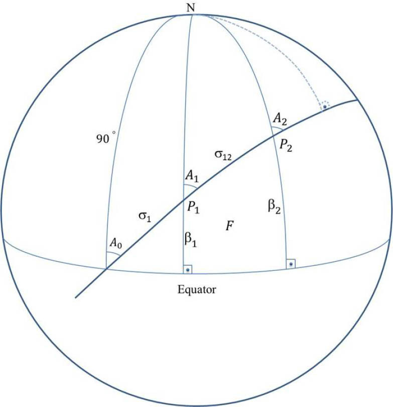
The F area in Figure 1 is calculated with the MATLAB code from Equations (2) and (3). Also, a, b, e and e′ are ellipsoid parameters. The solution of I1 integral in Equation (5) can be calculated using math computer software or the serial coefficients produced by Karney method. A0, A1 and A2 azimuths and the spherical geodesic line length are calculated by using spherical trigonometry in Equations (3–14):
Equal Area Projections
Maps can be produced using equal area projections to minimise area deformation, instead of Karney solution for area calculation on the ellipsoid reference surface. Large and medium-scaled topographic maps (1000–250,000) are produced using UTM or Lambert Conformal Conic (LCC) projection in the world. Area corrections (F – f) can be minimised with the selection of equal area projections. For calculating the area deformation, area correction formulas (F – f) calculated with the help of coordinates produced from the maps are presented to the users by using UTM and LCC systems. Area correction formulas (F–f) and area calculation on the ellipsoidal reference surface are not available in CAD and GIS applications. Therefore, instead of conformal projections, one of the projections that equal area projections should be selected for high accuracy calculation of a parcel area.
In this study, first, 15 forest parcels that varied between 300 and 3000 ha were selected within the boundaries of Kütahya Forest Regional Directorate (Figure 2). The area values of the 15 forest parcels selected in the study area were calculated with the equal area projections presented in Table 2 using GIS software. Thus, the most suitable equal area projection was determined by calculating the area deformations of the all projections (ITRF96 datum, 3° of longitude in width).
Figure 2
Satellite imagery of forest parcels (left) and geographical boundaries of the Kütahya Regional Directorate of forestry and forestry operation directorates in ITRF96 datum (right)

Table 2
Projections and parameters used in the study
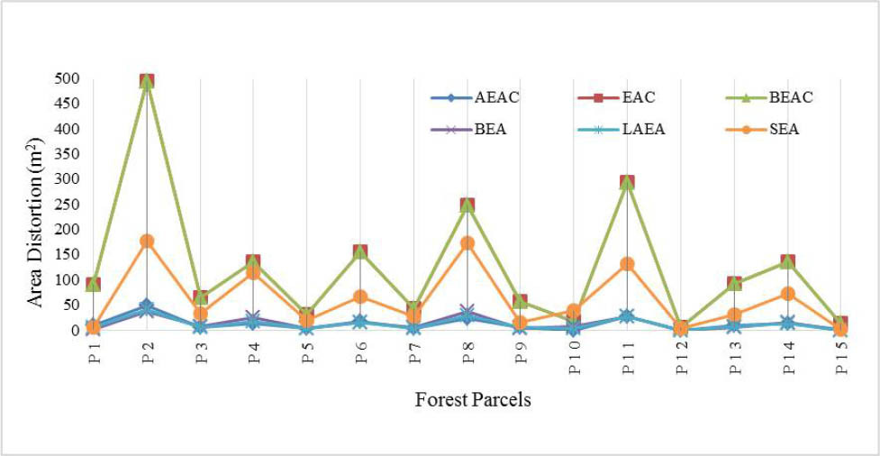
Areas of forest parcels were calculated by using the projections given in Table 2. At the same time, the areas of these forest parcels were calculated by the Karney method. The areas of the forest parcel calculated by the projections (Table 2) were compared with the areas calculated by the Karney method (Table 3). The distortion values are randomly distributed depending on the shape and size of the parcel and the distance of the parcel from the projection centre.
Table 3
Area distortions of equal area projections
In Table 3, area corrections are calculated for the all equal area projections. According to Table 3 and Figure 3, two types of projections (Albers Equal Area Conic [AEAC] and Lambert Azimuthal Equal Area [LAEA]) with the least area corrections were determined. One of these projections can be preferred. AEAC projection was selected in this study in terms of the ease of calculation and processing time.
The area distortions have been also examined by employing Karney method in UTM. Thus, it is investigated whether the area reduction formula (F – f) is sufficient in the UTM system. The area on the ellipsoidal reference surface can be calculated by adding the reduction formula (F – f) to the area calculated from the map. Area distortion formulas (F–f) are defined from the surface of the sphere and the non-concave shape in UTM. In conformal transformation, the deformation value is directly related to the size of the area and its distance to the y-axis (Grossmann, 1976):
where F, f, R, ym represent the area on the ellipsoid reference surface, the area calculated from the map, the Gaussian mean radius and the average distance from the y-axis (prime meridian) of the parcel, respectively. Area reduction value (F – f) of application parcels in UTM was calculated using Equation (15) (ym = 13 km, R = 6370 km). Area reduction values (F – f) of the parcels are given in Table 4.Table 4
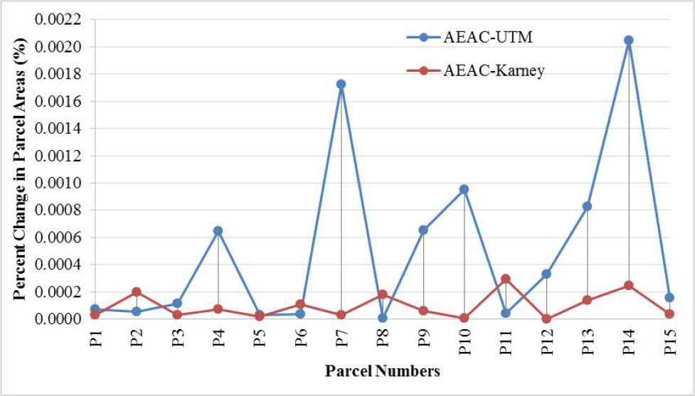
Comparison of UTM, area reduction (F – f), Karney method and AEAC projection
The area reduction values calculated from Equation (4) in UTM were compared with the results obtained from the Karney method. In the light of the results, it has been observed that the results obtained from the Karney method are more reliable (Figure 4).
Therefore, in order to determine the area distortion in large areas, it is necessary to calculate the area with geographical coordinates on the ellipsoid reference surface or to transform to equal area projections.
The area difference that was calculated by using the Karney method and AEAC projection varies from 1 to 50 m2. When comparing the parcel areas on the reference surface calculated using Equation (15) in UTM and AEAC projection, it has been found that there are differences from approximately 10 to 200 m2 for each parcel (Figure 4).
If AEAC projection was chosen instead of UTM, a total of 800 m2 distortion was observed in the total of all area distortion values in the parcels.
Area Corrections Caused by Map Scale
One of the important criteria in the area calculation is how the corner coordinates of the parcel are produced. In this context, the scale of the map where the corner coordinates of a parcel are produced is directly related to the area calculation of the parcel. Area calculations of the parcels, which cannot be measured in the terrain, are calculated on the scaled map. For this, the corner coordinates of the parcel are produced on a scaled map by digitisation technique. In this context, the larger the scale of the map produced in coordinate data, the higher the sensitivity values of the data produced on the map.
The area calculation performed using the parcel corner coordinates produced from the scaled map is formulated below:
where n, f and (x,y) denote the total number of corners of the parcel, the area of the parcel on the map and the corner coordinates of the parcel. The parcel area is calculated using Equations (16) and (17). Then the root mean square error (RMSE) of the parcel area is calculated using following equations: where mp and S represent the RMSE of the corner points and the square of the diagonal lengths of the parcel (Bogaert et al., 2005; Navratil and Feucht, 2008; Hejmanowska and Woźniak, 2009). Equations (18–20) are not available in GIS software. But users can add Equations (18–20) to the program with the help of the interface.It is seen in Table 5 that as the scale of the map gets smaller and the area gets bigger, the value of the area correction due to the scale increases as a result of digitisation technique. For example, an area of 2500 ha, which is calculated using the corner coordinates produced from a 25,000-scale map, has been calculated as an area of 2.5 ha. When the parcels with large areas (forests, pastures, etc.) are taken into consideration, it is clearly seen that the area differences resulting from the use of medium-sized maps have high values. The areas calculated from the data obtained from the scaled maps using the digitisation technique are given in Table 5.
Table 5
The effect of scale-related accuracy of measurement on the area (for regular polygon parcels)
On the other hand, smooth square parcels are used for the application in Table 5. When using 15 forest parcels selected within the study area instead of these parcels, the results obtained are shown in Table 6.
Table 6
The effect of scale-related accuracy of measurement on the area (forest parcels) in AEAC projection
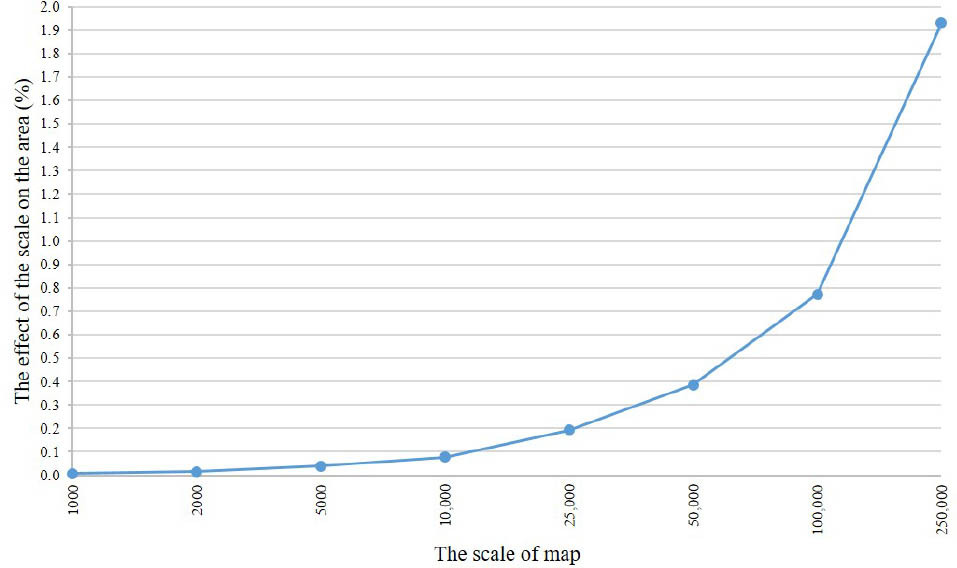
When these forest parcels are examined, it is seen that the effect of digitisation technique used in scaled maps increases as the scale of the maps gets smaller. Therefore, large-scale map must be used for the area calculation with the digitisation technique in the parcels with large areas (Figure 5).
Area Corrections Caused by Elevation and Slope Factors
Today, area calculations are made on the surface of the ellipsoid or projection plane with a conform transformation from the ellipsoid. The ellipsoid selected is the reference ellipsoid determined in the geodetic datum. GRS80 is used in ITRF datum and Hayford ellipsoid in ED50 datum. The ellipsoid selected as reference is determined by the geoid. Ellipsoidal height (h) is measured in Global Navigation Satellite System (GNSS) measurements. The height type shown on the maps is the geoidal height. The transformation between these two types of heights is enabled by geoid undulation (N). The effect of the height factor in the calculation of a parcel area is determined using Equation (21):
where Fh, F, havg denote the area of the parcel with a height from the ellipsoid, the area of the parcel on the surface of the ellipsoid and the average of the heights of the parcel corner points, respectively (Koçak, 1985). The slope factor is not taken into account in this calculation. Area correction of sample parcels with different heights and area values are shown in Table 7.Table 7
The effect of ellipsoidal height on area (for regular polygon parcels)
As seen in Table 7 and Figure 6, area deformations increase as the area and height values increase. When using 15 forest parcels selected within the study area instead of these parcels (for regular polygon parcels), the results obtained are shown in Table 8.
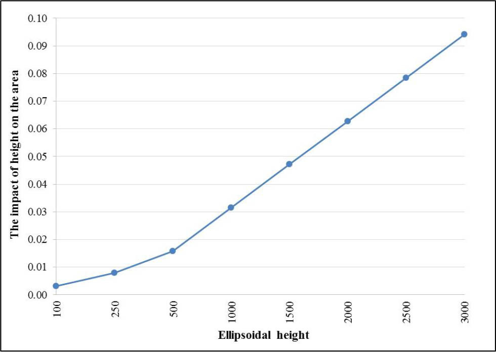
Table 8
The effect of ellipsoidal height on area (for forest parcels)
In the light of the results obtained in Table 8, it is observed that the area correction values increase as the average ellipsoidal height values of the parcels increase. Equation (18) that is formulated above is not available in GIS software. In applications that require high precision, GIS users should consider the height factor when using large areas of parcels.
In the calculation of the parcel areas, besides the height factor of the terrain, the slope of the terrain is an important factor to be taken into consideration. The effect of the slope factor on the area of the parcel with a certain height from the ellipsoidal reference surface is presented in Equation 22:
where Fh, F, tan a denote the area of the parcel with a height from the ellipsoid, the area of the parcel on the surface of the ellipsoid and the average slope of terrain, respectively. The changes caused by the effect of the slope factor on the area of the parcel are presented in Figure 7.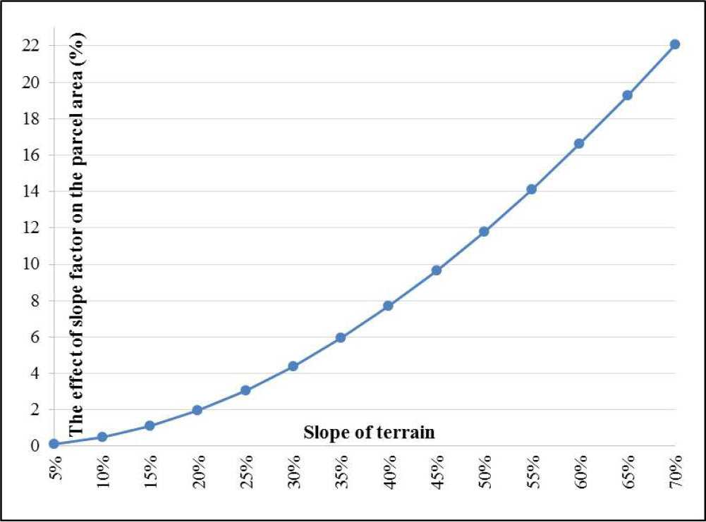
Area values calculated using scaled maps are not exact area values. In order to compute the exact area value of a parcel, different types of area corrections must be added to the area calculated from the scaled map. The impact of these area corrections on the area calculated on the scaled map is shown in Tables 5 and 6 as a percentage.
As seen in Table 9, area corrections calculated based on projection and scale factors have negative values and area corrections calculated based on other factors have positive values. The biggest correction to be added to the parcel area is the area correction caused by the slope factor.
Table 9
Rate of total area corrections
. Results and Discussion
In this study, the area corrections and their sizes to be added to the area value calculated from the scale map in GIS applications are examined.
There are many factors that affect the value of an area. These are selection of map projection, the scale of the map, the ellipsoidal height and the slope of the terrain. GIS users often neglect these area corrections in GIS applications or cannot predict whether area correction values are within the accuracy limits. In addition, since the services provided by users of GIS-based software are limited, such software is insufficient in calculating the area correction values.
In this study, GIS users are presented with the area calculation method (Karney method) on the ellipsoid surface that is not available in GIS software. In addition, it was observed that the GIS software was insufficient in the area correction calculation of the parcels with large area values in the UTM system. In addition, the issue of which of the equal area projection types will be used in GIS applications where the area value is important has been examined with the help of the GIS software. At the end of the test, AEAC projection type has been proposed.
Area information of a parcel is calculated using different methods. One of these methods is the area calculation using the digitised technique from the scale map. When using this technique, it is absolutely necessary to calculate the area correction based on scale. In this study, the area corrections to be added to the areas of large forest parcels according to the size of the map scale (1:1000–1:250,000) were calculated and served to the users.
Slope and elevation parameters are other corrections that affect the parcel area calculated from the scaled map. In this context, area corrections to be added to large forest parcels were calculated from the elevation (100–3000 m) and slope (5%–70%) parameters according to the selected value ranges.
The percentages of the change in all the area corrections are shown in Table 9 according to the parcel areas. In GIS applications where a parcel's area information is used, the required precision and accuracy values are an important point. In this context, it is necessary to produce data according to the request and needs of the user. For this reason, in the applications where the area information is important, the area corrections to be added to the area due to different parameters should be taken into consideration.
Selection of projection and slope of the terrain parameters are available for users in GIS software. However, due to the map scale and the height of the terrain, area corrections to be added to the parcel area are not available in GIS software. In this study, these area corrections obtained by using Equations (18–21) can be added to GIS software by users.
Today, there are many parcel area-based applications such as real estate valuation, land tax, farming support and cost–benefit analysis in GIS applications. In this context, it is necessary to calculate the area of the parcel precisely in order for such applications to give correct results. Therefore, in order to obtain the correct result in determining the exact area calculation of the parcel, it is necessary to take into account the selection of projection, scale of the map, elevation of the map and slope of the terrain factors.