
. Introduction
The extensive use of GNSS measurement techniques for levelling works requires knowledge of the geoid or quasigeoid course in the area covered by the works. Knowledge of the course of these surfaces allows for the integration of satellite measurements with ground levelling measurements in valid height systems. Classical realisation of a height datum through a network of benchmarks is increasingly being supplemented or replaced by models of geoid or quasigeoid determined on the basis of different types of data. The accuracy requirements for height determination in valid vertical datums require knowledge of an accurate geoid or quasigeoid model and sufficiently accurate ellipsoidal height determination by GNSS techniques.
In Poland, works on determination of geoid or quasigeoid models have been carried out for many years, a review of which is presented in Kryński (2014). To develop the models, gravimetric data from various sources, astro-geodetic data, levelling measurements and GNSS satellite measurements were used. For the territory of Poland, several models with estimated internal accuracy of a few to about a dozen centimetres were developed. Among them, there was the GUGiK’2001 model, the first national model made available for use in levelling works (Pażus et al., 2002). The currently valid quasigeoid model in Poland is PL-geoid2011 (Kadaj, 2014). This model was built as a result of local fitting of EGM2008-based quasigeoid to 570 points of the networks: ASG-EUPOS (including eccentric points), EUREF-POL, POLREF and EUVN. It is commonly used in GNSS receivers to determine normal heights on the territory of Poland, and was also implemented in the TRANSPOL 2.06 application program (Kadaj, 2014). The authors of the model estimate its standard error at the level of 0.015 m, and deviations at control points are in the range of −0.054 m to 0.066 m. Field test in the eastern part of the country showed disparity up to 2.7 cm from the model and satellite levelling (Borowski, 2015).
Szelachowska and Krynski (2014) presented a new gravimetric quasigeoid model for the territory of Poland, named GDQM-PL13. The mean Faye’s anomalies in a 1′ × 1′ grid, vertical deflections from the territory of Poland, gravity anomalies from neighbouring countries and the global geopotential model EGM2008 were used as input data. Height anomalies calculated from the GDQM-PL13 model were compared with the corresponding height anomalies obtained from satellite/levelling data at the POLREF, EUVN and ASG-EUPOS networks and at stations of a control satellite/levelling traverse, obtaining mean square errors below 2.2 cm.
Modelling of (quasi-) geoid course is the subject of studies undertaken in different countries. For example, Das et al. (2018) deals with a problem of modelling the local course of geoid in test areas in Papua New Guinea. The aim of the study was to use ellipsoidal and orthometric heights and – on their basis – to develop a local model of geoid with the use of various polynomial models. The third degree polynomial ensured the accuracy of the geoid model fit at the level of ±20 cm.
In the study of Falchi et al. (2018), a local quasigeoid model was developed for the area of north-western Italy, using the global EGM2008 model and height anomalies at points of the permanent stations’ network. Ordinary kriging interpolation was used to interpolate the values of the anomalies at unknown points. The study conducted in the area of 28,000 km2 showed that the use of the global model and only 25 height anomalies significantly improved the accuracy of results compared to the use of the global model itself.
As a result of the work presented in Morozova et al. (2019), a quasigeoid model for the western part of Latvia was introduced. The model was developed on the basis of GNSS/levelling observations, data from EGM2008, and astro-geodetic measurements of deflection of the vertical made by Zenith digital camera (DZC) and those calculated from the EGM2008 model. Quasigeoid surface modelling by finite element method was performed using DFHRS software (Jäger, 2013). It has been shown that the use of deflections of the vertical, both measured and calculated from the EGM2008 model, gives a significant improvement of accuracy of the quasigeoid model and facilitates the localisation of possible systematic errors, especially in mountainous areas.
In recent years, the problem of determining highly accurate local (quasi-) geoid models has been repeatedly addressed. Lamparski (2008) presented results from the development of a local geoid model on an area of over 1000 km2 near Olsztyn. The accuracy of the model was estimated to be better than 1 cm. The study of Trojanowicz et al. (2020) compared four approaches to local quasigeoid modelling using the global geopotential model EGM2008 and height anomalies obtained from GNSS measurements and levelling (two models) and the additional use of gravimetric data and a digital terrain model (two models). As a result of analyses performed in the south-west of Poland, comparable results were obtained in all the considered approaches. Differences emerged when the number of points with determined height anomalies and accuracy of the global geopotential model were reduced.
. Theoretical basis for the use of quasigeoid model in surveying
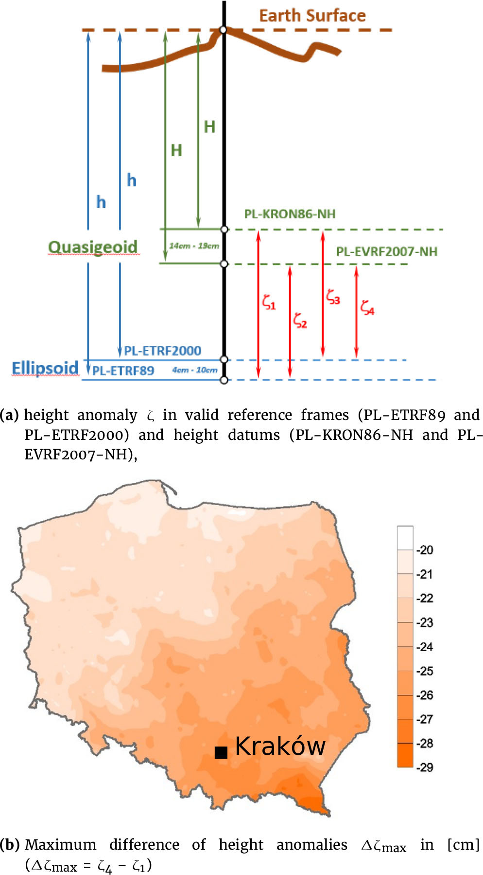
A quasigeoid model integrates ellipsoidal heights obtained by GNSS measurements and normal heights obtained by geometric levelling. The quantity that integrates ellipsoidal heights (h) derived by GNSS techniques and normal heights (H) derived by levelling is the height anomaly ζ (Figure 1a):
Values of height anomalies vary with position on the reference ellipsoid:
Spatial variation of ζ on a given area may be modelled, providing the opportunity of computing ellipsoidal heights or normal heights at arbitrary points according to the formulas:
Therefore, function (2) establishes a quasigeoid model (often referred to as a ‘geoid model’). Due to the differential nature of the height anomaly (1), the quasigeoid model does not lose its relevance due to, for example, deformation of the terrain surface, despite changes in the ellipsoidal or normal height. Therefore, together with satellite levelling, it can be an alternative to the vertical control network in areas subjected to such surface deformations.
In order to use a quasigeoid model to calculate heights, it is necessary to adapt it to a valid reference frame and height datum. In Poland, there are currently two reference frames: PL-ETRF89 and PL-ETRF2000, and two height datums: PLKRON86-NH and PL-EVRF2007-NH (Regulation, 2012, 2019). Hence, four quasigeoid models may be in use (Figure 1a). For example, the model ζ4 is adjusted to ellipsoidal heights and normal heights referenced to PL-ETRF2000 and PL-EVRF2007NH, respectively. The difference of ellipsoidal height of a point expressed in both PL-ETRF89 and PL-ETRF2000 reference frames varies between 4 cm and 10 cm, and the difference in normal height expressed in PL-KRON86-NH and PL-EVRF2007NH is between 14 cm and 20 cm (Figure 1a) (Kadaj, 2018). Therefore, the maximum discrepancies in the height anomaly are equal to almost 30 cm. Such discrepancies occur between models ζ4 and ζ1, and concern the southern regions of Poland (Figure 1b).
For levelling measurements, where the height difference between points A and B is the basic quantity, the formula (3) will take the form (5):
where: ζ hAB is the difference of ellipsoidal heights between points A and B, and the height anomaly increment ζAB is calculated from the quasigeoid model on the basis of the coordinates (φ, ζ) or (x, y) of these points.This way of handling the quasigeoid model is free from systematic errors resulting from the use of different reference frames and height datums. Possible discrepancies in height differences resulting from different tidal systems adopted in height datums may occur for very long levelling sections. The maximum discrepancy in the tide-free model that was used in PLKRON86-NH and the zero-tide model used in PL-EVRF2007NH does not exceed 1 cm on the section running meridionally throughout Poland (Borowski and Banasik, 2020).
. Project of a network of points for building a quasigeoid model in the area of Krakow
The quasigeoid model construction project concerned the area of the city of Krakow,1 that is, an area of approx. 20 km ×30 km in the south-eastern part of Poland (Figure 1b, Figure 2). One of the goals of constructing the model was to provide a more detailed course of this surface, currently represented by the national model PL-geoid2011. The base for this national model was the global geopotential model EGM2008 and selected points of primary control networks (Kadaj, 2014). Only three such points (two eccentric points of the ASG-EUPOS KRAW station and the POLREF network point) are located in Krakow.
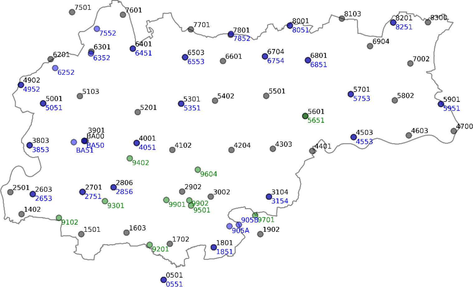
Figure 2
Location of the measurement points over the Krakow area. Points measured in the first campaign – grey, points measured in second campaign – blue, additionally measured points – green
Their uneven distribution across the city and a few tens of kilometres to the nearest points of the national model indicate that the national model within the area of Krakow may be less detailed. Moreover, diversified topography of the southern part of Krakow indicates a more varying course of quasigeoid in this area in relation to the northern part of the city.
The preliminary project of generating a quasigeoid model for the area of Krakow assumed that:
the base for the model will be several tens of points evenly distributed over the study area, height anomalies ζ will be determined in these points;
points will be evenly distributed over the entire area, and the distances between adjacent points will correspond to values of Δ ζ no greater than over a dozen centimetres (the maximum value of Δ ζ within the area of Krakow is about 4 cm/km, which is assumed to correspond to distances between points from 2.5 km to 5.0 km);
height anomalies will be computed on the basis of static GNSS surveys supplemented with levelling observations coming from referencing to an upgraded detailed vertical control network and benchmarks of the primary base vertical network; at least half of the points will be verified through additional GNSS and levelling measurements;
quasigeoid surface modelling will be carried out using the global geopotential model in valid reference frames and height datums, and its final form will be available as a regular grid; the values of ζ computed in nodes of this grid in accordance with the formula (2) will be used to interpolate ζ at any point with the known coordinates (x, y) or (φ, λ);
a model validation will be performed in selected areas, based on independent GNSS and levelling observations.
Considering the above project assumptions, a regular network of 50 points, located 3 km apart, evenly covering the area of Krakow, was generated. Using internet maps, three to five possible locations for the measuring point were selected for each point. The availability of signals from GNSS satellites and the shortest possible distance from the benchmark of vertical control constituted two selection criteria for a given location. The final location of a given point intended for GNSS and levelling observations was determined as a result of field reconnaissance. The spatial distribution of the so-designed measurement points, together with the points from repeated and verifying measurements, is shown in Figure 2.
. Characteristics of GNSS measurements and levelling data used to build a quasigeoid model in the area of Krakow
GNSS measurement was carried out for determination of the ellipsoidal height of selected points near the levelling benchmarks. For observations, at all measured points, uniform measuring equipment was used – dual-frequency GPS/GLONASS receivers (Leica GS16). The first survey campaign was performed in 17 static sessions 5 hours in length. The observation interval was 5 seconds and the elevation mask 0°. In each session, from 3 to 5 points were measured synchronously (Table 1).
Table 1
First survey campaign – sessions 1–17. Point selected for second measurement are in bold. Second measurement – sessions 18–24 (shaded grey)
Based on the data quality conducted with the teqc software, points affected by significant signal interference due to multipath, as well as points with horizon obstructed were eliminated from further processing. Post-processed points met the following criteria: number of recorded observations > 90%, RMS of the multipath error in code observations < 0.15 m, number of cycle slips per recorded observations < 1/400.
As a result of the quality control of the data from the first measurement and to ensure the re-determination of the ellipsoidal height of at least one point from each of the observation session, 25 points were selected for the second measurement. The second GNSS campaign was carried out in 7 static sessions, with the same equipment and the same receivers’ settings as in the first survey. The location of the measurement points over Krakow area are shown in the Figure 2.
The post-processing of the observations was performed in four different forms using commercial software and internet services. A list of variants of the post-processing is presented in Table 2.
Table 2
Post-processing variants
| Software | Solution |
|---|---|
| Leica Geo Office | Network solution, ASG-EUPOS reference stations (KRA1, PROS) |
| GNSS Solutions | Network solution, one ASG-EUPOS reference station (KRA1 or PROS) |
| AUSPOS (internet service) https://www.ga.gov.au | Network solution, EPN/IGS reference stations |
| MagicGNSS (internet service) https://magicgnss.gmv.com | Precise Point Positioning |
The ellipsoidal coordinates obtained were converted into the PL-ETRF2000 frame. Height anomalies ζ were calculated based on the arithmetic mean of the four solutions presented above. The mean values of ζ from all measured points were characterised by a standard deviation in the range of 1.9 mm–15.4 mm, which indicates a good agreement between the solutions. The accuracy of the measurement was verified by comparing the height anomalies determined twice at 23 points. Differences ζ from the two measurements are within −8.3 mm to −8.7 mm, with a standard deviation σ = 4.5 mm. On this basis, height anomalies calculated as the arithmetic mean of the four variants of the post-processing were adopted as the final results of the measurement.
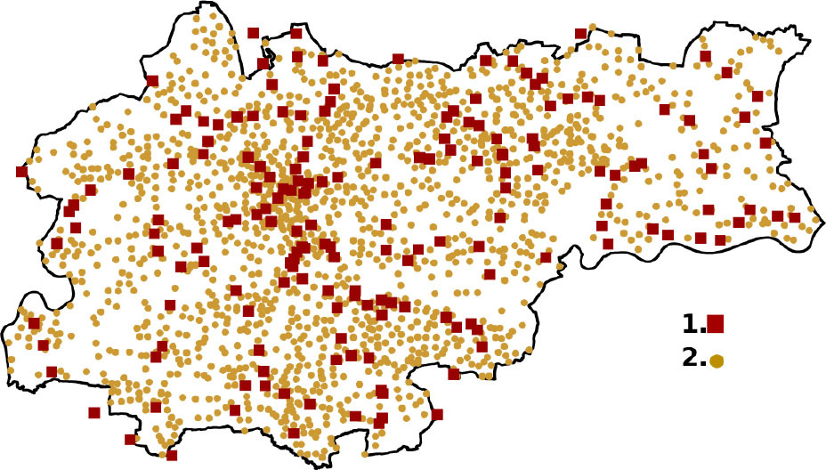
Normal heights of GNSS points being the basis of quasigeoid model were calculated with reference to the selected benchmarks of primary base and detailed vertical control networks (Figure 3). Detailed vertical control network within the area of Krakow was upgraded in the years 2016–2017. It consists of more than 1,800 wall and ground benchmarks, which gives an average density of 5.7 points/km2. This control network has been tied to more than 180 benchmarks of the primary base (former primary vertical control of the I and II class). The levelling observations were adjusted in the PL-KRON86-NH and PL-EVRF2007-NH vertical datums.
The appropriate location of the GNSS points in the vicinity of a benchmark of the vertical control allowed for a levelling tie of a point with the average accuracy of 1 mm, on a segment consisting of up to 3 level stations. For the purpose of developing a quasigeoid model, the heights of the benchmarks were subject to additional office and field verification. The aim was to check the network referencing benchmarks, whose current heights may have differed from the catalogue heights, and also, the height differences between referencing benchmarks were checked.
Verification rested on:
identification of GNSS points outlying from the preliminary quasigeoid model,
control measurements of levelling sections in the vicinity of the identified benchmarks,
re-adjustment of the levelling network (detailed control) after correction of height differences or elimination of the reference benchmark (the primary base control). The adjustment was carried out in two stages (free adjustment, multipoint adjustment) according to the procedure proposed by Osada and Gralak (2017). Extreme differences of the catalogue heights and those from the re-adjustment attain the values of −0.9 cm and +1.2 cm, and for 80% of the benchmarks, the differences did not exceed ±0.5 cm. Such a verification procedure allowed for increasing the accuracy of the normal height of GNSS points used to model the quasigeoid.
. Development of a quasigeoid model for the city of Krakow
To develop a quasigeoid model for the area of Krakow QuasigeoidKR2019, ellipsoidal and normal heights of 66 GNSS/levelling points were used in two reference frames: PL-ETRF89 and PL-ETRF2000, and two height datums: PLKRON86-NH and PL-EVRF2007-NH. The spatial distribution of the GNSS/levelling points used for modelling purposes is shown in Figure 4.
Figure 4
Spatial distribution of GNSS/levelling points for the construction of a quasigeoid model for the Krakow area

Whilst developing the local quasigeoid model, a high-resolution global geopotential model EGM08 (Pavlis et al., 2012) was used as a large-scale trend in height anomalies obtained from the GNSS/levelling measurements. The use of EGM08 has significantly contributed to the simplification of the (residual) height anomaly functional model in comparison to the models constructed on the basis of raw height anomalies. Thus, the local height anomaly model for the Krakow area is the sum of two components (for the i-th point):
The first component, ζEGM08, comes from the global geopotential model EGM2008 and it is interpolated from a regular grid covering the city of Krakow. The second one ζRES (residual height anomaly) is approximated by the following function (for the i-th point):
The above function was selected from several tens of tested ones, based on the following criteria:
simplicity – a small number of parameters defining the functional model,
meeting statistical criteria verifying the model – normality of model residuals, significance of model parameters, acceptable mean errors, satisfactory results of cross-validation technique.
To avoid numerical instabilities whilst developing the function approximating the residual height anomalies, the mapping of coordinates of the PL-2000 system on a unit square was applied, that is:
where:The assessment of the functional model of residual height anomalies was performed in two stages.
In the first stage – a classical analysis of model accuracy and outliers’ detection based on the residuals obtained from the least squares fit (internal accuracy, in-sample) was performed. The analysis of model residuals was preceded each time by a test verifying their normality; only those models for which all parameters were statistically significant were considered.
In the second stage – two variants of the cross-validation technique were used to assess the predictive capability of the model (external accuracy, out-of-sample): leave-one-out and random (Monte Carlo). The first one rests on a sequential removal of a single observation from the dataset, prediction of its value on the basis of a functional model built from the remaining data and a comparison with a reference value (previously removed). The second variant rests on a random removal of a given percentage of observations from the data set (20% adopted in this study), forecasting their values on the basis of the model built from the remaining data and comparison with reference values (previously removed), and such a procedure is repeated n-times (1000 repetitions adopted in this study).
Such an approach provides the opportunity for obtaining the accuracy characteristics of the prediction model, which is a hint of which model could claim to be the best among those examined. It also allows to assess the stability of the adopted functional model. In both cross-validation variants, the mean square error, mean absolute error, median and maximum cross-validation error were used. All the above mentioned characteristics are based on the differences between the observed values (removed) and the corresponding model-based predicted values.
The in-sample and out-of-sample accuracy characteristics of the residual height anomaly model indicated the need for eliminating 4 or 5 points from the data set, depending on the reference frame and height datum variant (absolute residuals/cross-validation differences greater than 15 mm but not exceeding 20 mm). Outliers were removed sequentially and each time a new model of residual height anomalies with full accuracy analysis was estimated.
The accuracy and agreement characteristics of the quasigeoid model QuasigeoidKR2019 with the measurement data for the reference frame PL-ETRF2000 and height datum PLKRON86-NH are shown in Table 3.
Table 3
Accuracy characteristics of the local quasigeoid model for the city of Krakow
The analyses showed that the height anomaly model fits the empirical data at the level of single millimetres, whereas if its accuracy is measured with the maximum prediction errors obtained from the cross-validation technique, it can be concluded that prediction uncertainty greater than 15 millimetres should not occur when using the recommended model. Similar conclusions can be drawn for the remaining variants of reference frames and height datums.
. Comparison of local QuasigeoidKR2019 model with national PL-geoid2011 model
In order to assess the gain resulting from the use of the local model (QuasigeoidKR2019) instead of the national one (PL-geoid2011), a comparison was made. In the comparison, GPS/levelling-derived height anomalies have been taken as a reference (total of 60 points). The comparison was made for the reference frame PL-ETRF2000 and height datum PLKRON86-NH. Figures 5 and 6 show the differences between the models in question and the measurement considered as the reference.
Figure 5
Difference of height anomalies derived from the national model PL-geoid2011 and GPS/levelling-derived ones

Figure 6
Difference of height anomalies derived from the local model QuasigeoidKR2019 and GPS/levelling-derived ones
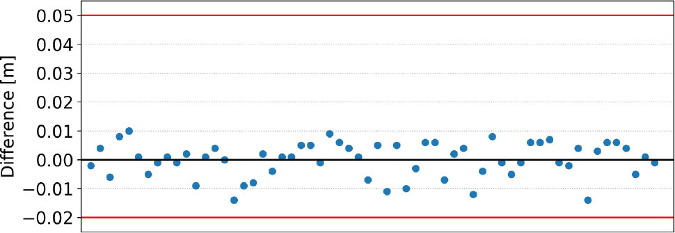
Inspecting both the above graphs, one can observe a significant decrease in differences between the local and national model in reference to the GNSS/levelling-derived height anomalies. The summary statistics for the two models are listed in Table 4. Comparison of two models with respect to GNSS/levelling height anomalies shows a triple reduction in values of individual quartiles and a mean absolute difference for the developed local model. These summary statistics clearly indicate that the accuracy of the local model for the city of Krakow is significantly higher than that of the national one.
Table 4
Summary statistics of absolute differences between models and GNSS/Levelling derived height anomalies
. Summary
The local model QuasigeoidKR2019 has been developed for the Krakow area, based on many-hours static, repeatable GNSS observations made at 66 points distributed throughout the Krakow area and normal heights obtained by referencing to the detailed vertical control network. The achieved repeatability of the height anomalies from two independent determinations at 22 points is within the interval (−0.0083 m; 0.0087 m), with a standard deviation of 5 mm. Such a verification is the basis for evaluating the quality of GNSS and levelling measurements. Height anomalies derived from observations’ processing were then used to develop an approximation function that models the residual course of a quasigeoid within the area of Krakow with respect to the global geopotential model EGM2008; planar coordinates in the PL-2000 coordinate system are the input arguments to the approximation function. On the basis of comparisons and accuracy characteristics, it can be estimated that the accuracy of the local model QuasigeoidKR2019 in the area of Krakow is higher than that of the national model PL-geoid2011. This is supported by the lower value of the extreme difference equal to 14 mm for the local model and 44 for the national model. The mean absolute difference is equal to 5 mm for the local model and 16 mm for the national model.